Computing Cross Sections with Different Broadening Parameters
In this tutorial, we create a cross section for a molecule using different broadening coefficients.
We again choose the CO Li2015 line list from ExoMol. We compute the cross section using ExoMol’s given \(\rm{H_2}\)-\(\rm{He}\) broadening files and also using 2 custom broadening methods. One of these custom broadening methods has a constant relationship between the pressure broadening Lorentzian half-width-half-maximum and the lower state rotational angular momentum quantum number (i.e. \(\gamma_{L}(J) =\) constant) and the other has a linearly decreasing relationship.
We strongly recommend reading the Quick Start guide if you have not done so yet.
Download CO line list and \(\rm{H_2}\)-\(\rm{He}\) broadening files from ExoMol
By now you should be a seasoned cultist of the Old One’s family, so you know what to do.
But this time, note that the summon function you’ve been using all this time has also been downloading pressure broadening files from ExoMol. In the input folder, you will see files for \(\rm{H_2}\), \(\rm{He}\), and air broadening (H2.broad, He.broad, and air.broad).
[1]:
from Cthulhu.core import summon

species = 'CO'
database = 'ExoMol'

# Download CO line list
summon(database = database, species = species)
 ***** Downloading requested data from ExoMol. You have chosen the following parameters: *****

Molecule: CO
Isotopologue: 12C-16O
Line List: Li2015

Starting by downloading the .broad, .pf, and .states files...
Fetched the broadening coefficients, partition functions, and energy levels.
Now downloading the Li2015 line list...

Downloading .trans file 1 of 2
100%|██████████| 1.40M/1.40M [00:00<00:00, 1.50MiB/s]
Converting this .trans file to HDF to save storage space...
This file took 0.3 seconds to reformat to HDF.

Downloading .trans file 2 of 2
100%|██████████| 63.5k/63.5k [00:00<00:00, 290kiB/s]
Converting this .trans file to HDF to save storage space...
This file took 0.1 seconds to reformat to HDF.

Line list ready.
Cthulhu’s Default Pressure Broadening
When you don’t specify a pressure broadening prescription (as we haven’t until now), Cthulhu will use a default treatment for pressure broadening. The default is as follows:
ExoMol: \(\rm{H_2}\)-\(\rm{He}\) pressure broadening with 85% \(\rm{H_2}\) and 15% \(\rm{He}\) (via the downloaded
H2.broadandHe.broadfiles).HITRAN / HITEMP: air broadening using a \(J\)-dependent set of broadening parameters computed by averaging over other quantum numbers in the HITRAN
.parfiles.VALD: a collisional approximation for \(\rm{H_2}\)-\(\rm{He}\) pressure broadening with 85% \(\rm{H_2}\) and 15% \(\rm{He}\).
You can of course always specify a different treatment, as we will see below.
Adding custom broadening files
Now, let’s create our custom broadening file and add them to the directory. To do this, we create numpy arrays for \(J\), \(\gamma_{L}(J)\), and \(n_{L}\) and write them to a file.
[2]:
import numpy as np

# Populate arrays
J = np.linspace(0, 80, num = 81)    # Rotational quantum numbers from J = 0 to J = 80
gamma_L_0 = 0.07 * np.ones(81)      # Lorentzian HWHM is 0.07 for all J
n_L = 0.5 * np.ones(81)             # Temperature exponent is 0.5 for all J
Now that we have defined the necessary variables, we call the write_broadening_file function to write these arrays to a file and place it in the correct folder. This function requires at least 5 parameters, the name of the file (broadening_file), the data to be written (data), the ‘input’ directory (input_dir), the name of the molecule (species), and the database (database).
The 3 arrays we just created should be combined into 1 array prior to calling the write_broadening_file function. This can be done using np.stack, as shown below. Make sure to keep the same order of the arrays (J then gamma_L_0 then n_L).
The variable input_dir should be set to ./input/ unless you have edited the file structure Cthulhu automatically creates.
[3]:
from Cthulhu.broadening import write_broadening_file

data = np.stack((J, gamma_L_0, n_L))  # Combine arrays into 1 array to pass into write_broadening_file function

broadening_file = 'constant.broad'    # Name of the file we will save data to

input_dir = './input/'                # Top level input directory that contains line list data for all species

# Create broadening file
write_broadening_file(broadening_file, data, input_dir, species, database)
Great, we have added our first custom broadening file!
Now let’s do the same for a broadening file where \(\gamma_{L}(J)\) decreases linearly for increasing \(J\) until a cutoff at \(J = 20\). The steps are the same, except gamma_L_0 will be different. For simplicity, we just redefine this variable, as well as the name of the broadening file, and keep everything else the same.
[4]:
gamma_L_0_beginning = np.linspace(start = 0.07, stop = 0.06, num = 21)         # 20 evenly spaced numbers from 0.07 to 0.06
gamma_L_0_end = 0.06 * np.ones(60)                                             # Lorentzian HWHM is 0.06 for all J after J = 20
gamma_L_0 = np.concatenate((gamma_L_0_beginning, gamma_L_0_end), axis = None)  # Combine both arrays for full Lorenztian HWHM

data = np.stack((J, gamma_L_0, n_L))  # Combine arrays

broadening_file = 'linear.broad'    # Name of the file we will save data to

input_dir = './input/'              # Top level input directory that contains line list data for all species

# Create broadening file
write_broadening_file(broadening_file, data, input_dir, species, database)
Computing and Plotting Cross Section
Now we are ready to compute the cross section. We do this in the usual way. The only parameter that changes is broad_type and broadening_file. If we set broad_type to ‘fixed’ a constant relationship between \(J\) and \(\gamma_{L}(J)\) is assumed. If we set broad_type to ‘custom’, the custom.broad file we added is used. If we assign no value to broad_type (or assign it to ‘default’), Cthulhu defaults to using the broadening parameters already downloaded with the line
list. In the case for CO, the default is H2-He broadening (as is often the case with ExoMol line lists).
Since we created 2 custom broadening files, we set broad_type to ‘custom’ in both calls to compute_cross_section. We also need to pass in the name of the broadening file in both instances, which you will recall were ‘constant.broad’ and ‘linear.broad’. As an aside, you can also set broad_type = ‘fixed’ for the constant \(\gamma_{L}(J)\) file we created.
[5]:
from Cthulhu.core import compute_cross_section

P = 1.0                        # Pressure in bars
T = 1000.0                     # Temperature in Kelvin
input_directory = './input/'   # Top level directory containing line lists

# Default H2-He pressure broadening
compute_cross_section(species = species, database = database, temperature = T,
                      pressure = P, input_dir = input_directory,
                      broad_type = 'default',
                      )

# Constant pressure broadening
compute_cross_section(species = species, database = database, temperature = T,
                      pressure = P, input_dir = input_directory,
                      broad_type = 'custom',
                      broadening_file = 'constant.broad',
                     )

# Linear in J pressure broadening
compute_cross_section(species = species, database = database, temperature = T,
                      pressure = P, input_dir = input_directory,
                      broad_type = 'custom',
                      broadening_file = 'linear.broad',
                      )
Beginning cross-section computations...
Loading ExoMol format
Loading partition function
Pre-computing Voigt profiles...
Voigt profiles computed in 5.0385457550000865 s
Pre-computation steps complete
Generating cross section for CO at P = 1.0 bar, T = 1000.0 K
Computing transitions from E2.h5 | 0.0% complete
Completed 6474 transitions in 1.8249874909961363 s
Computing transitions from Li2015.h5 | 50.0% complete
Completed 125496 transitions in 1.182199076996767 s
Calculation complete!
Completed 131970 transitions in 3.008382435000385 s

Total runtime: 11.12400327999785 s
Beginning cross-section computations...
Loading ExoMol format
Loading partition function
Pre-computing Voigt profiles...
Voigt profiles computed in 4.533660020002571 s
Pre-computation steps complete
Generating cross section for CO at P = 1.0 bar, T = 1000.0 K
Computing transitions from E2.h5 | 0.0% complete
Completed 6474 transitions in 0.07487936400139006 s
Computing transitions from Li2015.h5 | 50.0% complete
Completed 125496 transitions in 1.3549675960020977 s
Calculation complete!
Completed 131970 transitions in 1.4309075359997223 s

Total runtime: 8.964980600998388 s
Beginning cross-section computations...
Loading ExoMol format
Loading partition function
Pre-computing Voigt profiles...
Voigt profiles computed in 4.12634713800071 s
Pre-computation steps complete
Generating cross section for CO at P = 1.0 bar, T = 1000.0 K
Computing transitions from E2.h5 | 0.0% complete
Completed 6474 transitions in 0.06387955300306203 s
Computing transitions from Li2015.h5 | 50.0% complete
Completed 125496 transitions in 1.1314738929941086 s
Calculation complete!
Completed 131970 transitions in 1.1961962940040394 s

Total runtime: 8.202235151002242 s
Now we are able to plot the cross section. We need to first read the cross section files and add the cross sections to a collection.
[6]:
from Cthulhu.misc import read_cross_section_file, cross_section_collection

# Read in the cross sections we just computed
nu, sigma = read_cross_section_file(species = species, database = database,
                                    filename = 'CO_T1000.0K_log_P0.0_H2-He_sigma.txt')
nu2, sigma2 = read_cross_section_file(species = species, database = database,
                                      filename = 'CO_T1000.0K_log_P0.0_custom_constant_sigma.txt')
nu3, sigma3 = read_cross_section_file(species = species, database = database,
                                      filename = 'CO_T1000.0K_log_P0.0_custom_linear_sigma.txt')

# Generate an empty collection object for plotting
cross_sections = []

# Add first cross section to collection
cross_sections = cross_section_collection(new_x = nu, new_y = sigma, collection = cross_sections)

# Add second cross section to collection
cross_sections = cross_section_collection(new_x = nu2, new_y = sigma2, collection = cross_sections)

# Add third cross section to collection
cross_sections = cross_section_collection(new_x = nu3, new_y = sigma3, collection = cross_sections)
And finally we plot the results.
[7]:
from Cthulhu.plot import plot_cross_section

plot_cross_section(collection = cross_sections,
                   labels = ['H$_2$-He', 'constant', 'linear'],
                   filename = 'Different_Broadening_Types_for_CO',
                   y_min = 1.0e-30,
                   )
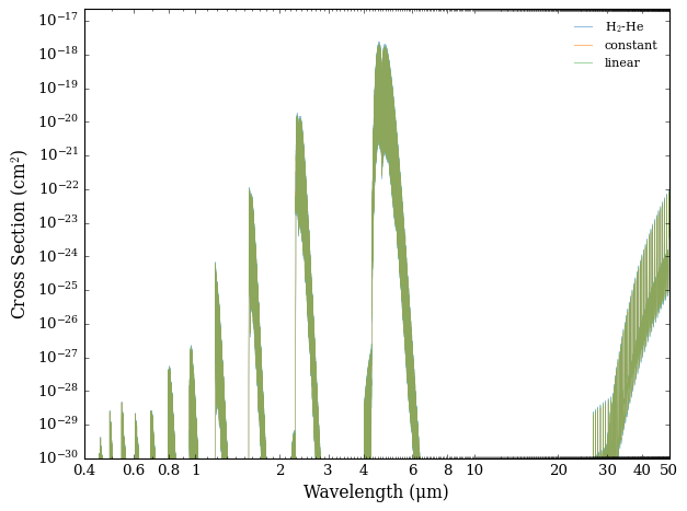
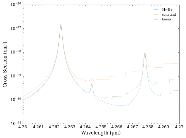
Whilst at first glance it may look like all three cross sections are the same, pressure broadening differences are easier to see when you zoom in on a narrow region.
Let’s examine the region from 4.26 μm and 4.27 μm to show the differences more clearly.
[9]:
plot_cross_section(collection = cross_sections,
                   labels = ['H$_2$-He', 'constant', 'linear'],
                   filename = 'Different_Broadening_Types_for_CO_Zoomed',
                   x_min = 4.26, x_max = 4.27,
                   y_min = 1e-31, y_max = 1.0e-26,
                   )