Cross Sections for Beginners
This notebook assumes you have followed the steps to download the Cthulhu package onto your local machine. If you haven’t, please visit the Installation page.
On this page, we run through the basic features of Cthulhu. We demonstrate how to download a line list, compute a cross section, and plot the result. Further tutorials are more nuanced and illustrate how to play around with various other features and advanced settings.
Downloading a Line List
Suppose we want to download the line list for CO from ExoMol. All of the major end-user functions are contained in Cthulhu’s core module, including the versatile (and powerful) summon function, which can automatically download line lists. At a minimum, all you need to do is specify the chemical species and line list database (e.g. ExoMol, HITEMP etc.).
The time has come. Let us summon Cthulhu!
Example: Downloading the CO line list from ExoMol
[1]:
from Cthulhu.core import summon     # Call forth the Old One

species = 'CO'             # Chemical species name
database = 'ExoMol'        # Line list database

# Download line list
summon(database = database, species = species)    # If you don't specify a line list name, a default line list will be downloaded
 ***** Downloading requested data from ExoMol. You have chosen the following parameters: *****

Molecule: CO
Isotopologue: 12C-16O
Line List: Li2015

Starting by downloading the .broad, .pf, and .states files...
Fetched the broadening coefficients, partition functions, and energy levels.
Now downloading the Li2015 line list...

Downloading .trans file 1 of 2
100%|██████████| 1.40M/1.40M [00:00<00:00, 1.89MiB/s]
Converting this .trans file to HDF to save storage space...
This file took 0.4 seconds to reformat to HDF.

Downloading .trans file 2 of 2
100%|██████████| 63.5k/63.5k [00:00<00:00, 302kiB/s]
Converting this .trans file to HDF to save storage space...
This file took 0.1 seconds to reformat to HDF.

Line list ready.
Notice how a specific isotopologue was chosen (Carbon-12 with Oxygen-16) for a default line list (Li2015). By default, the most abundant isotope combination on Earth is used (see the Isotope Tutorial for how to use other isotopologues). The default ExoMol line lists in Cthulhu generally follow the ExoMol project’s recommendations.
When summon is called, Cthulhu automatically creates an ‘input’ folder in the same directory as your .py file or Jupyter notebook. Various line list data files are then downloaded automatically for convenience (pressure broadening parameters, partition functions, and the state and transition files). Cthulhu reformats the ExoMol .trans files as HDF5 files to save storage space.
You can find the CO line list files in ./input/CO ~ (12C-16O)/ExoMol/Li2015.
Computing a Cross Section
We now have all the data needed to compute our first \(\mathrm{CO}\) cross section!
Import the compute_cross_section function, again from Cthulhu.core. This time, the user must specify at least five parameters, as opposed to the two for the summon function. As before, Cthulhu needs to know the species and database from which the line list was downloaded. Cross sections are computed at a certain pressure and temperature, so the user must specify the values P and T as well. Lastly, Cthulhu needs to know the top directory level containing downloaded
line lists. If no file structure has been changed by the user since the start of the tutorial, this will just be equivalent to setting input_directory = './input/'. This culminates in the code presented below.
Example: Computing CO Cross Section
[2]:
from Cthulhu.core import compute_cross_section

P = 1                          # Pressure in bar
T = 1000                       # Temperature in Kelvin
input_directory = './input/'   # Directory containing the line lists

# Calculate the CO cross section
compute_cross_section(species = species, database = database,
                      temperature = T, pressure = P,
                      input_dir = input_directory,     # Compute cross section has many more optional arguments and settings
                      )
Beginning cross-section computations...
Loading ExoMol format
Loading partition function
Pre-computing Voigt profiles...
Voigt profiles computed in 5.182578355001169 s
Pre-computation steps complete
Generating cross section for CO at P = 1 bar, T = 1000 K
Computing transitions from E2.h5 | 0.0% complete
Completed 6474 transitions in 2.0262211019999086 s
Computing transitions from Li2015.h5 | 50.0% complete
Completed 125496 transitions in 1.2598405160006223 s
Calculation complete!
Completed 131970 transitions in 3.2872161800005415 s

Total runtime: 11.539552496000397 s
As you can see, the console will display important information about how the computation is progressing. The Li2015 line list for \(\rm{CO}\) is quite small, less than 1 MB (corresponding to \(\approx\) 100,000 transitions), so the total cross section takes only about 10 seconds to produce. Larger line lists, like the POKAZATEL line list for \(\rm{H}_2 \rm{O}\), can be on the order of tens of gigabytes (\(\approx\) 6 billion transitions), and lead to cross sections that take around 24 hours to compute.
And that’s it! You’ll notice that an output folder has been created, at the same directory level as this notebook and the input folder. Navigate through the output folder (by clicking on the molecule, database, etc.) to find our \(\rm{CO}\) cross section in a .txt file titled CO_T1000K_log_P0.0_H2-He_sigma.txt. This is aptly named according to the parameters for which the cross section was computed.
The cross section file consists of two columns; the first is the wavenumber (in \(\mathrm{cm}^{-1}\)) and the second is the absorption cross section (in \(\mathrm{cm}^{2}\)). Some users may want to stop here, and just read in the cross section calculations for their own research. A function to read the cross section, read_cross_section_file, is provided and demonstrated below. Other users may want to plot the cross section for a more visually appealing final product. We show this as
well in the next section.
Reading in and Plotting a Cross Section
This section contains a basic introduction on how to use the plotting routine we’ve provided. For more complicated plots, like overplotting multiple cross sections on the same plot, see any of the other tutorials provided (like this one).
Example: Plotting \(\rm{CO}\) Cross Section
First, we want to return the wavenumber and absorption from the output cross section file. To do this, import the read_cross_section_file from Cthulhu.misc. This function requires the species and database as parameters, as well as the filename of the output file. We assign nu (the wavenumber) and sigma (the absorption cross section) to the return values.
[3]:
from Cthulhu.misc import read_cross_section_file

species = 'CO'
database = 'ExoMol'

# Read in previously computed cross section file
nu, sigma  = read_cross_section_file(species = species, database = database, filename = 'CO_T1000K_log_P0.0_H2-He_sigma.txt')
We’ll also need to import plot_cross_section and cross_section_collection.
[6]:
# Import relevant functions
from Cthulhu.misc import cross_section_collection
from Cthulhu.plot import plot_cross_section
Before we use plot_cross_section, we want to add our newly computed cross section to a collection. This extra step comes in especially handy for plotting multiple cross sections to one figure, but is still required even for one cross section. To do this, we call the cross_section_collection function, and pass in as parameters our return values nu and sigma.
[7]:
sigmas = []

# Add to collection
cross_sections = cross_section_collection(nu, sigma, sigmas)
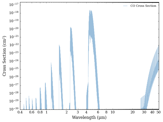
Then, to plot, call the plot_cross_section function. It requires at least 3 parameters: the cross section collection, an array of labels for each cross_section that is to be plotted (in this case we have added just one label), and a filename to save the plot to. Here, we have chosen a filename that describes exactly what cross section was plotted - the \(\rm{CO}\) cross section, from the Li2015 line list, at a temperature of 1000 K and pressure of 1 bar.
[8]:
# Plot cross section
spectrum = plot_cross_section(collection = cross_sections,
                              labels = ['CO Cross Section'],
                              filename = 'CO_Li2015_T1000_P1',
                              y_min = 1e-30)
In a newly created plots folder, which is at the same directory level as input and output, you’ll see the PDF file containing this plot.